



15 Techniques to lower the cost of AI
Incorporate smart harnesses, multi-model routing, self-hosting open-weight models, prompt caching, and SLM training to lower your AI spend.
AI budgets approved in the last two years have grown exponentially. A16Z indicates that its grown 3x year-over-year on a per-employee basis.
Figure 1
Everyone is spending more on AI, but some a lot more than others
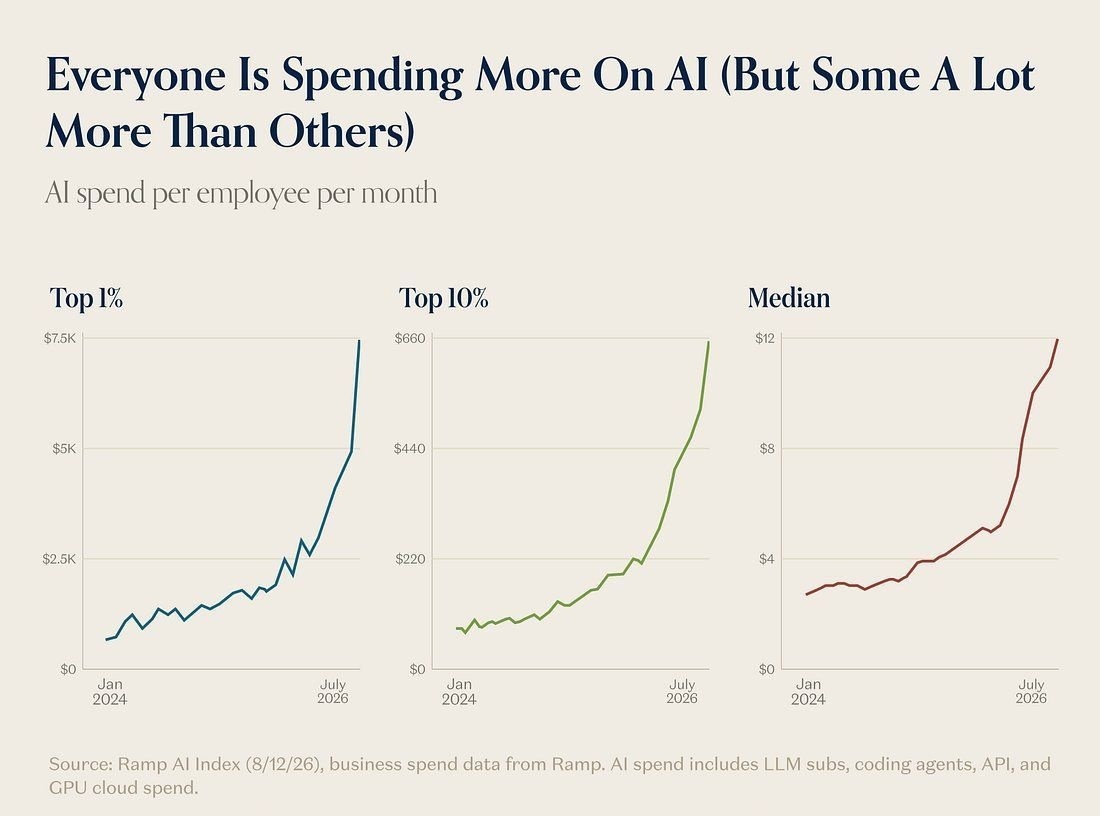
While many frontier model providers are subsidizing token spend for enterprises, this will not happen indefinitely and many enterprises are developing strategies for reducing their AI spend:
- Self-hosting open-weight models.
- Multi-model routing with prompt compaction and low model leverage.
- Training SLMs against proprietary to create small LORA adapters.
- Start with creating a system for observing, controlling, and routing all AI traffic across all providers.
- Assess your cost per user, per session, per task, and per AI provider.
- Execute over a dozen strategies that lessen your dependence upon expensive frontier models.
Unit prices are falling and bills are rising
Over the last three years, token prices have dropped roughly 90% each year. But, the total spent per employee has been tripling each year.
Andreessen Horowitz calls the price side LLMflation. For a model of equivalent capability, cost per token falls by roughly an order of magnitude each year. OpenAI cut GPT-5.6 Luna 80% on 30 July 2026, from $1.00 and $6.00 per million tokens to $0.20 and $1.20.
Figure 2
The price of a token falls while the demand behind it multiplies
Gartner put worldwide generative AI spending at $644 billion for 2025, up 76.4% on the year before. Andreessen Horowitz and OpenRouter studied more than 100 trillion tokens of production traffic and found the platform moving from roughly 10 trillion tokens a year to over a trillion tokens a day by late 2025.
As token consumption has increased, various efforts to measure the cost per task have emerged. Anthropic reports that a multi-agent system consumes roughly fifteen times the tokens of a chat interaction. Reasoning models and tool-calling loops cause a similar amplication. Every time there is a price cut against tokens, new multi-agent use cases and longer execution loops become commercially viable. In other words, as tokens get cheaper the type of work that AI can do grows.
Uber published its own accounting in August 2026 and wrote the arithmetic out:
total spend = users × sessions/user × turns/session × requests/turn × tokens/request × price/token
Figure 3
Uber's decomposition of what an AI programme spends
While the price / token is the baseline for calculating total cost, the design of your AI system and the type of AI behaviors will drive how many total tokens to be consumed.
Between February and August 2026 Uber's weekly active users across agentic tools grew sevenfold and weekly agentic requests grew 9.4 times. Over the same period, cost per thousand model requests fell 34% from its peak and cost per session fell 52% from its June peak.
Every time AI gets more efficient, the demand for it leaps, causing costs to keep rising.
Managing your AI costs is becoming an imperative, and there are numerous techniques available for lowering your AI spend.
The techniques that lower AI spend
Procurement moves the price per token. Every other technique moves one of the five terms in front of it: how many turns a session runs, how many requests a turn issues, how many tokens a request carries, and how often the same work is paid for twice.
- Procurement: Buying more tokens for less money
- Semantic response caching
- Multi-model routing: cascade and escalation
- Planner and worker role binding
- Sticky sessions and the prompt cache discount
- Prompt compression
- Memory compaction
- Smart harnesses: code execution instead of tool-calling loops
- Guardrails that stop requests
- Training specialist models into SLMs
- Self-hosting open-weight models
- Durable execution: not paying twice for a failed run
- Collapsing separately metered services
- Scale-to-zero on idle capacity
- Measuring cost per verified task
Every technique after the first one requires engineering work, and your workload sets how much each one returns. A business with uniform, repetitive traffic has more available than a larger business with varied traffic. Document reading repeats far more often than software authoring. You can measure the repetition in your own traffic before any engineering starts.
Figure 4
What one interaction consumes once orchestration is added
Technique 1 - Procurement: Buying more tokens for less money
Most procurement programs will execute disciplined acquisitions with model providers: annual commit tiers, batch pricing, reserved capacity, and a negotiated rate against a consumption expectation.
With vendors dropping costs unexpectedly, enterprises can attempt to incorporate Most Favored Nation and auto-ratchet price drops into their terms.
A commit tier applies to consumption nobody has examined. A workload spending twice what it needs to buys the discount on the waste along with everything else.
Technique 2 - Semantic response caching
A semantic response cache embeds each incoming request, searches the store of prior request embeddings for one within a similarity threshold, and returns the stored answer when it finds one. A "cache hit" costs an embedding call and a vector lookup, but no model tokens are spent as the LLM call is avoided.
Your cache hit rate tracks how repetitive your traffic is. The more similarity of your traffic, the higher the cache hit rate, and the larger the token benefit becomes. For example, support and FAQ workloads, where the same question arrives repeatedly, can have cache hit rates of up to 80%. Mixed application traffic like a coding session with a software engineer may only reach 15%. Personalised or time-sensitive traffic will have an extremely low cache hit rate, because stored answers will rarely match the incoming request.
Systems that provide semantic response caching let you define the threshold for a cache hit or miss. A loose threshold will find many matches, but you are increasing the likelihood of providing a cached answer to a question that wasn't asked. A tight threshold will force an exact-match cache. You will then have to periodically measure the false-hit rate on sampled traffic in order to tune the threshold to its optimal settings.
Technique 3 - Multi-model routing: cascade and escalation
Cascade routing sends your request to a 'cheap model' first, runs a correctness check on the answer, and re-issues the request to a frontier model when that check fails. The check can be a schema validation, a test run, a retrieval-grounding score, or a small judge model.
Your "escalation rate" is the share of cheap answers that fail, and it decides whether cascading returns anything at all. The cheaper it is to check an answer, the lower your escalation rate will be, and the more cascading will save you. Tasks with a deterministic check, like a schema validation or a compiler or a test suite, may escalate as little as 10% of the time. Tasks that you have to check with a judge model will often escalate 30% to 50% of the time. Tasks whose failures are expensive to detect will escalate often enough that cascading returns nothing.
Cascading will raise your total token consumption, because an escalated request pays for the cheap attempt and then pays again for the frontier attempt. If your cheap model is priced near a tenth of the frontier model rate and escalations to that frontier model occur 30% of the time, your savings from the 70% of requests that don't escalate can be up to 60%.
You can also use cascade policies with a multi-model router to escalate between two equivalent models in terms of capability. Those two models could have different pricing structures or rate limits that cause you to escalate away from the default choice. You can also use cascade and escalation policies to address provider outages, which let you escalate to another provider if there is an API outage. And, this author, has certainly been frustrated at the many API outages that we experience with Anthropic.
Technique 4 - Planner and worker role binding
Role binding assigns a model per turn rather than per task. The "planning turn", which decomposes the work and selects the steps, keeps your strong model. The "worker turns", which execute each step against a fixed instruction, go to a cheap model.
The longer your agentic runs are, the more worker turns they will contain, and the more this technique will save. A coding agent that plans once and then edits twenty files may run 80% to 90% worker turns. A conversational agent that calls one tool per reply will often run under 50%.
If your worker model is priced near a tenth of the frontier model rate, your savings across the 85% of turns that are worker turns can be up to 76%. Single turn traffic will not generate any meaningful savings.
You will give back the token savings on any worker turn that requires judgement, because those will fail on the cheap model and escalate back to the frontier model, which moves the workload toward cascade economics. So, the techniques that you use to identify which requests are planning turns and those that are worker turns can have a large impact on the savings that you will witness. One simple role binding is to assume new session requests are planning requests and subsequent requests in the same session are worker turns.
You can also bind roles more finely than a two-way split. For example, summarisation turns, tool-selection turns and format-conversion turns are all mechanical enough that a cheap, low effort model can satisfy the request as capably as an expensive model.
Technique 5 - Sticky sessions and the prompt cache discount
A conversation with an LLM provider consists of turns, or exchanges, between the consumer and the provider. Every piece of data in this exchange has to be converted into tokens, which are the main unit of billing for providers. Providers can cache these tokens as a way for them to save on compute costs and that savings is typically passed along to the consumer by charging less for cached tokens than for freshly minted ones.
The parts of this conversation that can be reliably detected as cached is called the "stable prefix". This can include system instructions, tool schemas, retrieved documents, and more. You pay less when these are read from a provider's "prompt cache" instead of generating new tokens.
Cache eviction on a hosted provider is driven by conversation idle time against the time-to-live (TTL), and misses are usually caused by prefix instability, a timestamp or per-user field ahead of the breakpoint, or a prefix that never clears the model's minimum threshold for caching.
If you're self hosting models, then you can know and optimize the size of the cache (e.g. vLLM supports this). For hosted providers, there is no way to know the capacity of the cache. Instead you need to optimize for cache hit rate. Each provider exposes session cache hit metadata in their own way.
Sticky session routing in an LLM conversation should always be a reasonable default, which also ensures maximum cache hits. The longer the conversation is, the better the cost savings on the prompt cache. If the conversation is short or so much time passes between turns that it exceeds the TTL, then you'll likely see little to no savings from caching.
A cached stable prefix bills at about a tenth of the normal input token rate, so your savings across the stable portion of your prompt can be up to 90%. A conversation that carries a 20,000-token fixed prefix and 500 tokens of new input per turn can see most of its input bill disappear from the second turn onward.
Cache writes cost more than normal input tokens, so the time-to-live that you choose is itself a cost decision. Uber reports a 1.25x premium for a five-minute entry and twice that for a one-hour entry. At the 2x premium an entry has to be read at least once more inside its time-to-live before it breaks even. One simple time-to-live policy is to set it to the median gap between turns that you already see in your traffic, and to raise it only for the session types that reliably come back.
You need to be particularly careful if there is a load balancer or non-sticky router between the consumer and the LLM endpoint, as this could easily negate all cache-related cost savings by swapping endpoints mid-session.
Technique 6 - Prompt compression
A "compression pass" runs your prompt through a small model that rewrites it to preserve the information the task needs on fewer tokens. It runs ahead of the frontier model call, and it adds its own inference cost, though many organizations mitigate that cost by self-hosting the compressor model.
The more redundancy or unnecessary prose your prompt carries, the more it will compress. Retrieval-heavy prompts that carry long documents can compress by 20% to 30%. Instruction blocks and prompts that are already lean will not generate any meaningful savings, and a compression pass on those may cost you more than it saves.
One simple compression rule is to compress any retrieved document above a token count that you set, and to leave your instructions and everything under that count alone.
At 25% compression, your savings across the half of your traffic that carries long context can be up to 25% of those input tokens.
Just like any other part of an agentic system, this needs to be measured. Compression is lossy, so you should compare the results you obtain with compressed vs. uncompressed prompts before turning it on in production where poor compression can impact answer quality.
Technique 7 - Memory compaction
Memory Compaction rewrites accumulated session history into a shorter summary once your context passes a threshold. Without it, a conversation re-sends its full history on every turn, so your tokens per turn will climb linearly and your tokens per session will climb at a rate related to the square of the turn count.
The longer your sessions run, the more compaction will save you. Sessions of 50 turns or more can drop 40% to 70% of their session tokens, and that figure keeps growing with length. Sessions under about 10 turns (depending on the turn size) will not generally show any meaningful savings.
One simple compaction trigger is to compact once the context passes half the model's window, summarising everything except the last few turns. What compaction drops will not come back, so you will also have to pin the facts that the task cannot lose outside the compacted region.
Memory compaction and prompt compression are very different things that act on different inputs. Compression rewrites the prompt that a single request carries. Compaction rewrites what the session has accumulated behind it. Compaction and compression are not mutually exclusive.
Technique 8 - Smart harnesses: code execution instead of tool-calling loops
A "tool-calling loop" returns each tool result to the model and then takes another turn. A "code execution harness" gives the model a runtime and a library of functions instead, and the model writes one program that loops, filters and aggregates without returning to the model between steps.
The more steps in any given session that don't need to involve your model, the more a code harness will save you. Uber measured one database query issued through a tool-calling loop against the same query issued as code: 1,431,594 tokens against 900. Multi-step data work of that shape can see token savings of 60% to 95%. Work that needs model judgement at every step is less likely to generate meaningful savings.
Filtering, sorting, joining, counting and format conversion are all work that a runtime does for free and that a model charges you tokens to do badly. So, one simple harness change is to give the model a sandbox with your data clients already imported, and let it write one program instead of taking a turn per row.
In Uber's measurements, tool schemas loaded into every session added a further 50,000 to 70,000 tokens of overhead before any work began, and every turn re-sent them. If you load schemas on demand from a tool index rather than placing them in the system prompt, that overhead becomes a single lookup.
Technique 9 - Guardrails that stop requests
A "guardrail" evaluates a request against your policy before it reaches a model and rejects the ones that fail. Types of guardrails can include prompt-injection classifiers, PII detection, topic and jurisdiction rules, and much more. This kind of guardrail typically runs on a small classifier or a rule engine.
The savings here is the full cost of the run that each rejected request would have started, which on an agentic workload is many turns. Internal traffic may reject only 1% to 3% of requests while public-facing traffic can reject 5% to 15%.
Guardrails on the output side will cost you more than they save, because your tokens are already spent by the time that check runs. Their value is typically regulatory rather than fiscal.
You can also put budget guardrails in the same place. A cap on turns per run, a token budget per session, and a ceiling on tool calls per turn will each stop a runaway loop that no policy classifier would notice. An agent that reasons its way into calling the same tool four hundred times is a dangerous path to a very expensive day.
Technique 10 - Training specialist models into SLMs
A "specialist model" is a small, open-weight base that you fine-tune on your own graded traffic for one task by distilling the frontier model's outputs and applying reinforcement learning against your grades. It serves that one task, and everything else routes to your general model.
Your share of eligible traffic resides in repeating task clusters with checkable output. The more of your work that repeats, the more a specialist can save you. Document extraction, classification and structured generation can run 40% to 70% eligible for redirection to the specialist model. Open-ended authoring will often run under 15%.
A tuned specialist consumes about 40% of the prior input tokens and returns about 60% of the output length, on a model priced near half the frontier model rate. So, your savings across that eligible traffic can be up to 80%. A tuned 4B open-weight model can run at up to 12× lower inference cost than a frontier API on the task it was trained for.
One simple way to find your first specialist is to cluster a month of traffic by task and take the largest cluster whose output you can check automatically. You can use simple embedding that doesn't require a frontier model in order to detect these clusters. Below about 20% eligible traffic, your training and serving cost will exceed what you save.
You can also train more than one specialist and route among them. A second specialist on your second-largest cluster costs you another training run and no additional serving complexity, because the router is already there from the cascade work.
Figure 5
The cost of not implementing AI optimization
Training a specialist on the work that repeats will save you more than four times what prompt compression saves at those assumptions. Every figure moves with your own workload. If you have no multi-turn traffic you will earn nothing from sticky routing, and if your work never repeats you will earn nothing from a specialist model.
Technique 11 - Self-hosting open-weight models
Every hosted provider sells you tokens at a published rate. When you self-host, you stop buying tokens and start buying compute. You rent or own GPUs, you serve an open-weight model on them, and your effective price per token is the GPU-hour cost divided by the number of tokens that hour actually produced.
That division is the whole story. A busy GPU produces a lot of tokens in an hour, and each one is cheap. An idle GPU bills the same hour and produces nothing, so every token it did produce carries the full cost of the hour. This is why utilisation, rather than the model you picked, sets your unit cost.
Reserved capacity held above roughly 60% utilisation can undercut metered frontier APIs on high-volume steady traffic. Below about 25% utilisation, metering is generally cheaper, and you will have converted a variable cost into a fixed one.
One simple break-even check is your GPU-hour cost divided by the tokens per hour that you can actually serve, set against the metered rate for the same class of model.
Throughput per GPU-hour is therefore the number to optimize, and continuous batching moves it further than any other single change at this layer. Serving stacks such as vLLM and SGLang implement this along with paged attention and prefix caching, which lets one node keep many requests in flight against a single set of weights. Quantisation buys more of the same, at a quality cost you should measure on your own tasks rather than take from a benchmark.
You should also count the operational cost that sits alongside the GPU bill. Model updates, capacity planning, and on-call for an inference tier are real work, and none of it appears in a per-token comparison.
You can also self-host only part of your traffic. Cascade routing, role binding, and your specialist models all route to the same cheap tier, and that tier carries the most volume at the lowest margin. Self-hosting it while your frontier calls stay metered gives you the utilisation you need without the commitment a full migration asks for.
At five trillion tokens a year against a frontier API baseline, with open-weight models served on reserved capacity and every technique above applied, the unoptimised route costs $31.09M and the optimised route $4.60M, a reduction of 85%.
Technique 12 - Durable execution: not paying twice for a failed run
An agentic workflow is a sequence of steps, and every completed step has already cost you tokens. If the process running it dies at step nine of twelve, the question is what happens to the nine steps you paid for.
Durable execution answers that by journaling each step as it completes. The state of the run lives outside the process, so a restart reads the journal, sees that nine steps are done, and continues at ten. Without it, the run starts over, and you pay a second time for work that already succeeded.
The longer your runs are, the more each failure destroys. Long agentic workflows that fail 5% to 15% of the time can recover 3% to 10% of their token spend. Short single-call tasks will not generally show any meaningful savings, since there is little completed work to lose.
One simple journaling boundary is the tool call. If you write state after every completed tool call, a restart repeats at most one step.
Replay only works if the steps are safe to repeat, e.g., side-effect-free/idempotent. A model response that has already been journaled is never re-issued, but a tool call that wrote to an external system may well be, so any step that touches the outside world needs an idempotency key or a check before it runs again. This is ordinary distributed systems design, and it is the part that tends to get skipped when the workflow is written by an agent framework rather than designed.
Where you keep that state shows up on the token bill too. An external store that answers in 150 to 200 ms adds delay, and an agent that is waiting will often re-ask the model for context it already had. State held in the runtime and read in under 10 ms removes that round trip.
Technique 13 - Collapsing separately metered services
Every service in your architecture that handles a request has its own meter and its own unit. That is normal and, by itself, not a problem. The problem is capacity. Each service is provisioned for its own peak, independently of the others, so one burst of traffic is paid for once at every meter it crosses.
Running an agentic workload on AWS bills against fifteen separately metered services, each on its own unit: per token, per state transition, per tool call, per policy decision, per record stored, per evaluation, per shard-hour, per KPU-hour.
Table 1
The AWS services that are needed to build an agentic system
| Chargeable item | How it is metered |
|---|---|
| AgentCore Runtime | Per vCPU-hour, per GB-hour |
| AgentCore Memory | Per record stored, per retrieval |
| AgentCore Gateway | Per tool call, per tool search |
| AgentCore Observability | Per GB ingested into CloudWatch |
| AgentCore Policy | Per policy decision |
| AgentCore Evaluations | Per evaluation |
| Bedrock model inference | Per token |
| Bedrock Guardrails | Per text unit |
| Bedrock Model Distillation | Per training run |
| AWS Step Functions | Per state transition |
| DynamoDB, Aurora | Per request, per GB |
| ElastiCache, MemoryDB | Per node-hour |
| Kinesis, MSK, SQS, SNS | Per shard-hour, per message |
| Managed Flink | Per KPU-hour |
| EventBridge, EventBridge Scheduler | Per event, per invocation |
Those peaks do not arrive together. A queue sized for its worst minute and a database sized for its worst minute are both mostly idle the rest of the time, and you are holding both. The more meters a request crosses, the more of that headroom you carry.
One simple audit is to take a single production request, trace it, and list every service that bills for it along with the unit each one bills on. The list is usually longer than the team expects, and no individual line looks unreasonable, which is why this cost survives review.
Running agents, memory, orchestration, streaming, and endpoints on one runtime collapses those meters into one and provisions the headroom once, and your infrastructure cost can fall by up to 90% against an assembled stack carrying the same volume. This is infrastructure spend rather than tokens, and it sits beside your model bill rather than inside it.
Technique 14 - Scale-to-zero on idle capacity
Reserved compute bills whether or not it is doing anything. Scale-to-zero releases it when no request is in flight and restores it when the next one arrives.
What you save is the idle share of your own traffic, which is a property of your users rather than of your architecture. A workload that follows business hours in a single region may idle around 70% of the week. The same workload spread across time zones will idle far less. One simple idle measurement is to bucket a week of request timestamps by the hour and count the hours that carried no requests at all.
Cold start is the constraint. Bringing capacity back takes time, and on anything with an interactive latency budget that time is visible to a user. The usual answer is a warm minimum: keep enough capacity running to absorb the first requests and let everything above it scale to zero. Your reduction then applies to the capacity above that minimum rather than to all of it, and the same traffic histogram tells you where to set it.
Batch and asynchronous work carries no such constraint and can go to zero without a warm floor, which makes it the first place to apply this. And scaling to zero does not mean scaling small: the same deployment can carry a peak of 10 million agentic transactions per second and then return to zero afterwards.
Technique 15 - Measuring cost per verified task
You cannot tell whether any of the previous fourteen techniques worked by reading a token bill, because a token bill counts what you spent and not what you got for it.
Cost per verified task is the correction. It is your total spend on a task divided by the number of runs that passed evaluation. Everything you spent stays in the numerator: the failed runs, the retries, the tokens the evaluation itself consumed, and the human hours an escalation took. Only the runs that produced an acceptable answer count in the denominator.
Consider what that catches. You move to a model priced 30% lower per token, and your pass rate falls from 85% to 50%. Your token spend drops, every dashboard you own reports a saving, and your cost per verified task has risen about 19%.
You instrument it by tagging every run with a task ID and an outcome, and then dividing. The tagging is straightforward; the outcome is the hard part, because it has to come from an evaluation you trust enough to act on.
The techniques that trade accuracy for price fail this most often: cascade, role binding, compression, and specialist models. Uber reports cost per merged pull request, cost per review, and cost per alert, each carried alongside a quality signal such as revert rate or mean time to resolution.
You can also carry the same denominator per team and per project. A cost per verified task that is rising in one team and falling in another will tell you something that an aggregate token bill never will.
This technique reduces nothing on its own. It tells you whether the other fourteen did.
The cost of agentic rework
Agentic systems attract rework because you have to make structural and architectural decisions about how agents are going to run before you understand how the workload will behave. You have to make decisions about where agentic state resides, how a failure is handled, and which services carry end user traffic.
The software around your AI models carries additional cost, and if you have to redesign those services after learning about the workload's behavior, then you have to incur an engineering rework cost. Industry measurement puts the loss to rework at ~20% of capacity.
Akka's agentic SDK takes an opinionated approach to system design. Effectively, if the AI system compiles and completes its testing, then it's production-ready without additional code changes. You will still have to tune the system against its evaluations, but the agentic system design is ready and capable of scaling with resilience.
Where to start
The first thing that you do is measure your token consumption and spend. Decompose your spend the way Uber does, into users, sessions per user, turns per session, requests per turn, tokens per request, and price per token.
AI and model gateways are equipped with the tools necessary to collect and measure these elements. Akka provides our own agent gateway with observability, token measurement, costing analysis, and optimization impact. Not only will we show you what your AI token spend is, but we will also show you the token savings that come from the different optimization techniques that you have activated.
After you get a measurement baseline, identify the types of techniques that are likely to have the biggest benefit for your workloads. We have a couple of calculators here and here on our Web site that can help you estimate what impact optimizations will have in total tokens and dollars saved.
How Akka can help lower your AI bill
The Akka Agentic AI Platform is designed to scale AI efficiently across diverse dev teams, projects, and geographies while lowering token costs and enforcing policies.
Figure 6
The Akka Agentic AI Platform
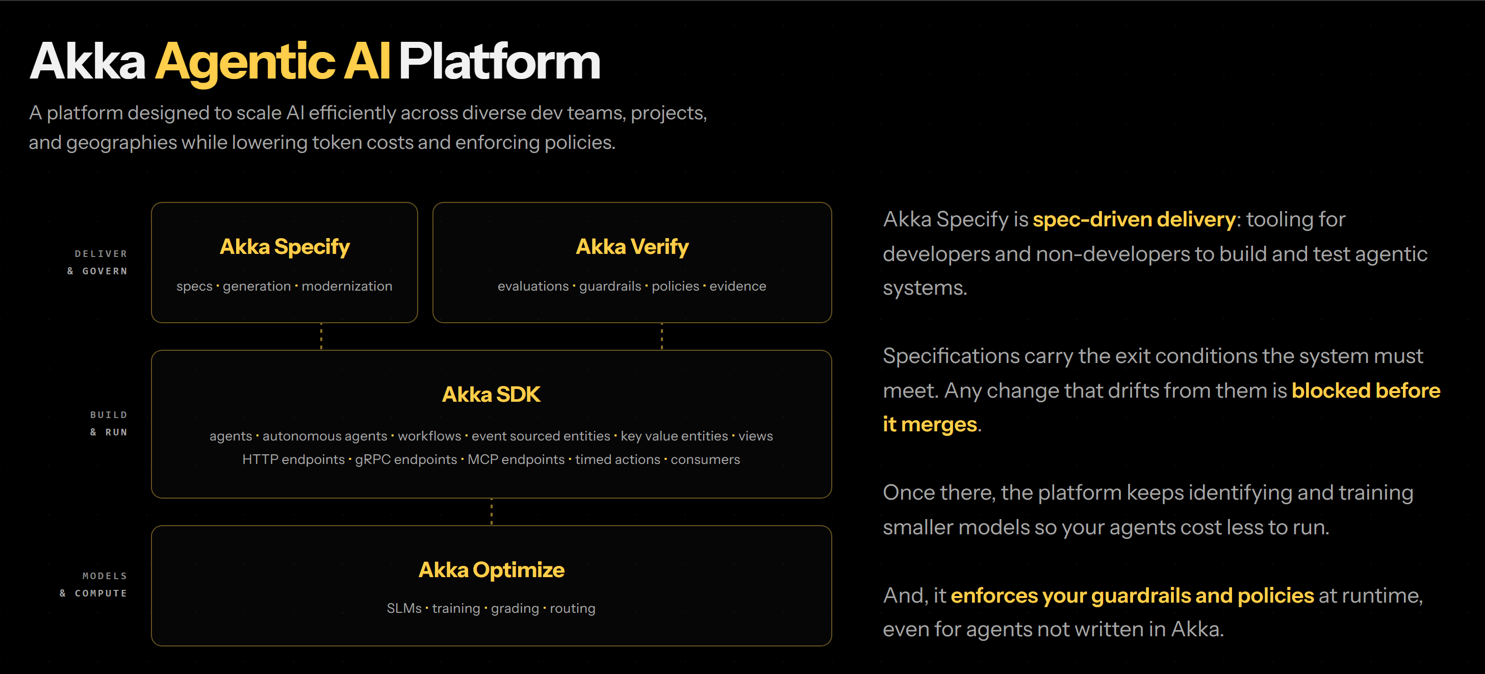
Akka Specify is spec-driven delivery: tooling for developers and non-developers to build and test agentic systems. Specifications carry the exit conditions the system must meet before any AI is releasable. Any change that drifts from them is blocked before it merges. Once there, the platform keeps identifying and training smaller models so your agents cost less to run. And, it enforces your guardrails and policies at runtime, even for agents not written in Akka.
The Akka Agentic AI Platform carries all of the components necessary for managing your AI traffic and lowering your AI bill.
Figure 7
An integrated platform that guarantees resilience and scalability
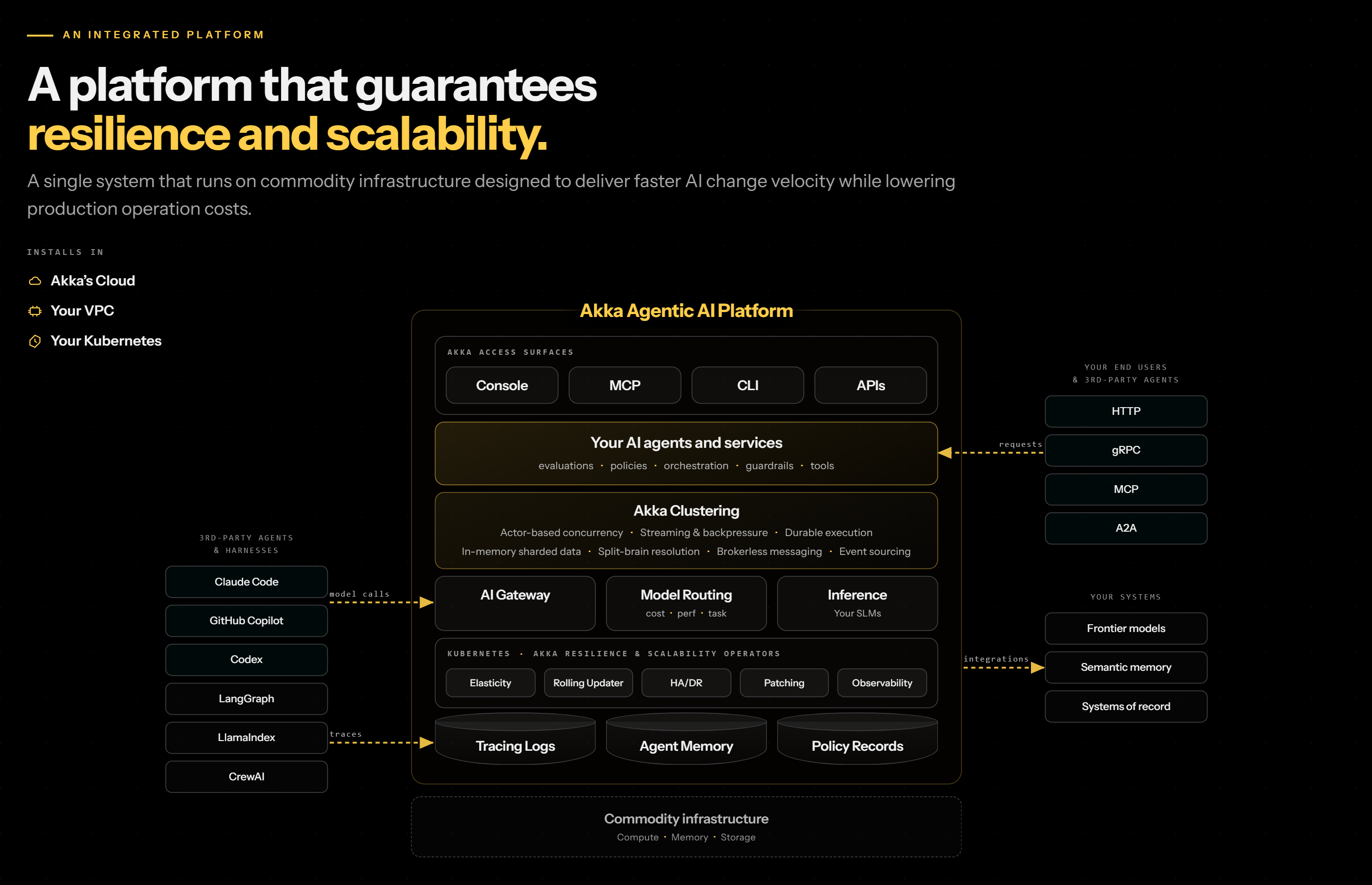
Table 2
Akka's platform provides a comprehensive set of AI optimizations for sovereign systems
| Technique | Akka offering |
|---|---|
| Semantic response caching | Akka Optimize |
| Multi-model routing: cascade and escalation | Akka Optimize |
| Planner and worker role binding | Akka Optimize |
| Sticky sessions and the prompt cache discount | Akka Optimize and Akka SDK |
| Prompt compression | You build this yourself |
| Memory compaction | Akka SDK |
| Smart harnesses | Akka SDK |
| Guardrails that stop requests | Akka Verify |
| Training specialist models into SLMs | Akka Optimize |
| Self-hosting open-weight models | Akka Optimize |
| Durable execution | Akka SDK |
| Collapsing separately metered services | Akka SDK |
| Scale-to-zero on idle capacity | Akka SDK |
| Measuring cost per verified task | Akka Optimize and Akka Verify |
Akka's platform is a single system that runs on commodity infrastructure designed to deliver faster AI change velocity while lowering production operation costs. This means that you can do more with AI and lower your overall AI bill.
To get the same capabilities of Akka, you need to integrate numerous, high-margin, meter-based services. Akka delivers higher performance and lower costs by only using AWS commodity infrastructure.
Table 3
What you pay for, with and without Akka
| AWS chargeable item | Without Akka | With Akka |
|---|---|---|
| AgentCore Runtime | Per vCPU-hour, per GB-hour | Included |
| AgentCore Memory | Per record stored, per retrieval | Included |
| AgentCore Gateway | Per tool call, per tool search | Included |
| AgentCore Observability | Per GB ingested into CloudWatch | Included |
| AgentCore Policy | Per policy decision | Included |
| AgentCore Evaluations | Per evaluation | Included |
| Bedrock model inference | Per token | Included |
| Bedrock Guardrails | Per text unit | Included |
| Bedrock Model Distillation | Per training run | Included |
| AWS Step Functions | Per state transition | Included |
| DynamoDB, Aurora | Per request, per GB | Included |
| ElastiCache, MemoryDB | Per node-hour | Included |
| Kinesis, MSK, SQS, SNS | Per shard-hour, per message | Included |
| Managed Flink | Per KPU-hour | Included |
| EventBridge, EventBridge Scheduler | Per event, per invocation | Included |
| EKS | not needed | Per cluster-hour |
| EC2 | not needed | Per instance-hour |
| EC2 GPU | not needed | Per accelerator-hour |
| RDS | not needed | Per instance-hour plus storage |
| S3 | not needed | Per GB stored and per request |
Akka AI spend calculators
We publish two calculators that prices a year of agentic AI on a hyperscaler stack vs. the same AI workloads running on an Akka stack. At five trillion tokens a year, graded at 80% on the hyperscaler and 80.2% on Akka, the hyperscaler cost is $8.09M versus the Akka stack costing $1.67M.
The Hyperscaler Savings Calculator will let you plug in your own numbers to estimate your likely savings.
We have another calculator, the Sovereign Savings Calculator, that let's you identify which optimization techniques to apply for your workloads, and how those savings could benefit your spend against the frontier models.
Talk to us about a plan for lowering your AI spend.